0. Introduction
- Two major features of recent math curricula are
- * the increased emphasis on functions throughout secondary school, and
- * their multiple representations: numerical, graphical, and symbolic.
These changes are motivated in part by the availability of electronic graphers, and in part by sound pedagogical thinking: different representations are more accessible to different students, and the ability to switch representations both reflects and facilitates depth of understanding for all students. I very much support these changes. (See for example the article A New Algebra, and the graphing calculator lessons on this site.)
One underused representation of functions, which I have found educationally rich, is the one with parallel x and y axes. I heard about it in a talk by Martin Flashman. I was inspired to develop some lessons for the textbook I co-authored with Anita Wah (Algebra: Themes, Tools, Concepts -- ATTC), using the name "function diagrams" for that representation.
On this page, I introduce function diagrams, and provide a number of lessons and activities to use them at various levels in secondary school. Of course, this is meant to complement, not replace other approaches to these ideas. Indeed, function diagrams are essentially a pedagogical tool, while the other representations of functions have a power and reach that make them life tools.
1. Basics
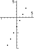
A function is a way to assign a single y value (an output) to each x value (input). It can be thought of as a set (perhaps infinite) of ordered pairs (x,y). In secondary school, we work mostly with functions on the real numbers. For example, the function y = 2x - 3 can be looked at in tabular, numerical form:
| x | y |
| 3 | 3 |
| 2 | 1 |
| 1 | -1 |
| 0 | -3 |
| -1 | -5 |
| -2 | -7 |
| -3 | -9 |
The (x, y) pairs listed on the table can also be represented as points on a Cartesian graph:
This worksheet can be used to introduce the basic idea of a function in these two representations: Guess My Function
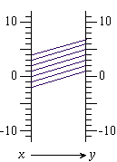
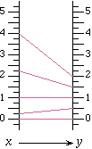
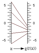
A function diagram is yet another representation, with parallel x and y axes. Each (x, y) pair is represented by a line segment connecting the input point on the x axis to the output point on the y axis. The line segment is called the input-output line. (In some cases, it is preferable to draw the whole line, instead of just a line segment. See "The Focus" below.)
Note that while on a cartesian graph one can show as many points as one wants, a function diagram becomes illegible if too many input-output lines are drawn.
In general, do not ask your students to spend too much time drawing function diagrams: it is tedious, and not all that enlightening. There may be exceptions to this, but it is usually more effective for students to analyze existing diagrams, to discuss diagrams you create on the overhead projector, or to use computers or calculators to create the diagrams.
Electronic Tools: A good discussion of function diagram basics can be had with this animation. See the function diagram applets page for more animations, and the function diagram software page for GeoGebra files, Cabri figures, and TI calculator programs you can download.
- Downlad these PDFs, to use when introducing function diagrams to your students:
- the table, graph, and function diagram for y = 2x - 3 (as above)
- blank tables and function diagrams
2. Operations
Middle School
One way to motivate many of the rules for operations with signed numbers is to generalize from patterns that work for positive numbers. For example:
3 + 3 = 6
3 + 2 = 5
3 + 1 = 4
3 + 0 =
3 + (-1) =
3 + (-2) =
3 + (-3) =
3 + (-4) =
Another way to think about this pattern, is to recognize the function 3+x=y, which can be represented by a function diagram:
It is easy to figure out how the diagram can be extended, and thus to fill out the rest of the pattern.
Similar methods can be used to explore other patterns of this type, thus motivating the rules for signed number arithmetic, and providing students with a way to reconstruct them on their own.
Beginning Algebra
Download Nine Function Diagrams, a worksheet slightly edited from the ATTC Teachers' Resource Binder.
Teacher's Notes: This is a rich activity, which can generate discussion about signed numbers, inverse operations, opposites and reciprocals, the use of symbols... It deserves plenty of time, perhaps two class periods. Before answering the questions, students will need to figure out the formulas for each diagram -- many find it useful to first make tables of values. Diagram f is the most difficult, and you can allow students who have trouble with it to temporarily skip it.
The worksheet sets up a crucial review of fundamental concepts of arithmetic, and of basic algebraic notation, in a novel format. The novelty makes for a lesson that is accessible and interesting to a wide range of students. The concepts reviewed include the following:
- A letter can represent a negative number, whether or not it is preceded by a minus sign
- A letter can represent 0 or 1
- It is possible to add and end up with a smaller number
- Adding a number is equivalent to subtracting the opposite, and vice versa
- It is possible to multiply and end up with a smaller number
- Multiplying by a number is equivalent to dividing by its reciprocal, and vice versa
These ideas are not explicitly addressed in the questions, but they are necessary to a full understanding of the answers. It is the teacher's responsibility to bring those out in class discussion.
Note that some students are surprised or even resentful that two consecutive questions could have the same answers as each other. That is a good opportunity to explain that what makes an answer correct is its mathematical validity, not such an incidental feature as whether it is the same answer as the previous one.
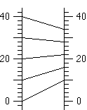
Solving Inequalities
Another potential use of function diagrams is to clarify the logic behind the rules one uses when solving inequalities by hand. For example, we know that -3<4. If we add -2 to both sides, we get -5<2, which is still true. However if we multiply both sides by -2, we get 6<-8, which is false. This is dramatically illustrated by the function diagrams for y=x+(-2) and y=-2x:
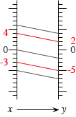
After looking at a few such examples, it is not hard to see that it is legitimate to add or subtract the same number on both sides of an inequality, and likewise to multiply or divide by a positive number. However multiplying or dividing by a negative number requires changing the direction of the inequality.
3. Functions
Definitions
- These basic ideas about functions can be visualized with the help of function diagrams.
- A function assigns a unique output to each input.
- The domain of a function is the set of its inputs.
- The range is the set of its outputs.
Magnification
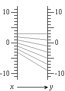
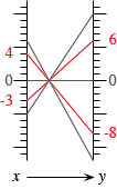
Any interval in the domain is "magnified" by a continuous function into an interval in the range. The magnification is the factor by which we multiply the directed length of the x interval to get the directed length of the corresponding y interval.
For example, in the first diagram below, the magnification is 2 for any x interval. However in the second diagram, the magnification depends on the selected x interval. For example, for the x interval from 0 to 4, the magnification is 1/2, however for the x interval from 1 to 4, the magnification is 1/3.
The magnification is constant only for linear functions. (We will discuss this in more detail below.)
Of course, magnification is just another word for the rate of change of the function. Slope in a cartesian graph and magnification in a function diagram are two representations of the same underlying idea (rate of change), and are calculated in the same way. But using different terminology in different contexts has some pedagogical value: it allows students to approach the concept afresh in a different context, and gives them a chance to make the connections themselves.
A fun activity is to do the "function diagram dance": move your hands vertically, in a physical representation of x and y, and have students guess the magnification. (Obviously, this cannot be very accurate, but you can distinguish values of m that are less than -1, equal to -1, between -1 and 0, equal to 0, between 0 and 1, equal to 1, and greater than 1.) After doing some examples, have students do the dance for values of m you choose.
- Download a transparency master / worksheet to discuss domain, range, and magnification. Choose among two versions:
- Six Function Diagrams -- Suitable for Algebra 1 or Algebra 2
- Eight Function Diagrams. -- This version requires familiarity with radians, trig functions, and natural logarithms, and thus is suitable for the end of Algebra 2, Precalculus, or the beginning of a Calculus course.
- Applets:
- Use Name That Function! (an online version of "Eight Function Diagrams") to discuss domain, range, and magnification.
- Use this magnification applet to explore rate of change for various values of Δx on a function diagram.
Composition
The composition of two functions is shown with linked function diagrams. For example:
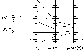
Here is the resulting function:
Questions for discussion:
- How was the function diagram above obtained from the linked diagrams preceding it? What formula corresponds to it? How could this formula be obtained from the original two?
- Given a function, is there a function that can be composed with it (in either order) to yield the identity function? If there is such a function, it is called the inverse function. What is the inverse function of f?
- How is the diagram of the inverse function related to that of the original function?
- How is the magnification for the composite function related to the magnification for the two functions we are combining? [It is the product of the magnifications. This relationship is a crucial concept in calculus (the chain rule) and function diagrams provide what must be the clearest way to explain it.]
Download a worksheet about composition and magnification, based on the figures above.
- Applets:
- Animation of composition of two functions, as above.
4. The Focus
The remaining activities are about the function diagrams of linear functions. In those diagrams, all the input-output lines meet in a single point callled the focus, or else they are all parallel, and the focus is a point at infinity.
Download the worksheet Focus on Function Diagrams and the figure Sixteen Function Diagrams. Together they constitute a lesson from ATTC, intended for use later on in an Algebra 1 course, or as review in a subsequent course. An alternative to students doing the whole lesson on paper is to have them work on #5 in small groups, then to have class discussions of the ideas in #1-4 and #6-20, and finally to have students do #22 individually, perhaps as homework. This could take two or three days, but it is time well spent, as it provides another way to think about familiar ideas that are sometimes remembered mechanically.
Note that the lesson described above assumes without proof the existence and uniqueness of the focus. Download the teacher worksheet Geometry of Function Diagrams, which addresses this question with the help of geometry.
In the case of linear functions, the focus contains all the information about the function, while individual ordered pairs are represented by lines. This is exactly the dual of the situation in a Cartesian graph, where individual ordered pairs are represented by a point, and the whole function is represented by a line. This leads to an interesting application of function diagrams. A system of linear equations in two variables can be solved graphically by seeking the intersection of two lines. In a dual fashion, the same system can be solved graphically by joining the foci of the two functions. The resulting line (if it exists) represents the unique ordered pair solution of the system. The cases where there are no solutions or an infinite number also have a clear representations with function diagrams. Download Representing Linear Functions, a lesson from ATTC on this duality.
- Applets
- This one-linear-function function diagram applet allows you to move the focus, and see the corresponding equation.
- This two-linear-function function diagram applet allows you to solve a system of two linear equations in a new graphical way. The same figure can be used to discuss the location of the focus for a given m, or for a given b. Finally, one can use it to visually approximate the inverse function for a given linear function.
5. History and Bibliography
I learned about function diagrams many years ago at the Asilomar meeting of the California Math Council, from Professor Martin Flashman, who (among other things) teaches calculus at Humboldt State University. He calls function diagrams "transformation figures" or "mapping diagrams". For what I call input-output lines, or in-out lines, Flashman uses "arrow", which is easier to work with, and carries almost as much information.
As far as I know, the first use of function diagrams to explain the chain rule is in Sherman Stein's Calculus and Analytic Geometry (1977). In there, he uses the metaphor of slide projectors, in what is almost certainly the origin of the term "magnification" to refer to rate of change. Flashman took this representation a lot further, applying it to the study of many functions, and making it a central part of what he calls sensible calculus.
I got the term "focus" from Abraham Arcavi and other Israeli researchers, who used function diagrams (which they called PAR -- parallel axes representation) in their work with math teachers. (Interestingly, as far as I know, not with students. Indeed, even if teachers never introduce this representation to their students, they gain some understanding from thinking about it themselves.) See Arcavi, Abraham and Rafi Nachmias (1989) "Re-exploring familiar concepts with a new representation." Proceedings of the 13th International Conference on the Psychology of Mathematics Education, 3, 174-181.
When I showed Paul Goldenberg my Cabri (now GeoGebra) function diagrams applets some years ago, he told me he had created a horizontal version, under the name dynagraph, long before I became interested in this. His idea was to give students a tactile experience, allowing them to see what happens to the y when you move the x -- a dynamic view, with a single in-out line, as opposed to looking at the overall diagram with many in-out lines. Of course, both approaches have a place. There is a dynagraph implementation in Geometer's Sketchpad.
I got the idea for using function diagrams to explain the rules about solving inequalities from "Effective Instruction", by Amy L. Nebesniak, in The Mathematics Teacher, Vol 106, No. 5, Dec 2012/Jan 2013.
To my knowledge, the only secondary school curriculum that includes function diagrams is Algebra: Themes, Tools, Concepts by Anita Wah and Henri Picciotto, Mountain View, CA: Creative Publications, 1994. The book is available for free download on this Web site: see below for a link and a list of the function diagram lessons. Of course, those are complemented by the activities on this Web site.
- Related pages on this site:
- Presentation slides (PDF | Keynote)
- Electronic tools for function diagrams
- Function diagram applets
- The geometry of y=mx+b
- Iterating linear functions
- Related lessons in Algebra: Themes, Tools, Concepts
- 2.7, 2.8, 2.9, 3.2, 3.10, 3.C, 5.1, 5.7, 8.2, 9.5, 12.7, 12.8
- Related article in NCTM's online journal:
- Delving into Functions with Function Diagrams
Subscribe to my newsletter